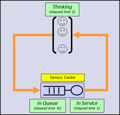
Let us consider a fixed (closed) population of users interacting with a service center, as shown in the following picture below:
- At t=0, an user arrives to the service center,
- From t=0 to t=W the user waits in the queue if all the servers (or workers) are busy at t=0, W is the wait time.
- At t=W one server gets free and takes the user for servicing him.
- From t=W to t=W+S and the server gives him the requested service. S is the service time.
- At t=W+S the user exits the service center after having being serviced.
- From t=W+S to t=W+S+Z the user remains out of the service center. Z is called the think time.
- At t=W+S+Z the user goes to step #1. that is, he arrives again at the service center, and the cycle repeats.
The think time (Z) is a measure of the user activity. It typically is much greater than the Service Time (Z>>S). For example, in SAPS benchmarks Z=10 s and S is about tens of milliseconds. In the context of SAP system sizing high activity users are assigned a Z=10s, medium activity users Z=30s, and low activity users Z=300s.
A quantitative approach
The fundamental question we would like to answer is: what is the response time (R) when the user population is N? That is, what is the relationship between the response time and the number of users R=R(N).
To focus on principles, and to keep things simple, let's derive R(N) with the simplifying assumptions:
- S is constant,
- Z is constant.
- m=1 (It is easily generalizable to an arbitrary number of workers).
Light Load Phase
Let us suppose there is only one user, that is, total population number is equal to one (N=1). The lone user arrives to the service center, never queues, receives service, departs, is away, and comes back to the service center. This loop is periodically repeated, being the period Z+S (the time it takes the user to cycle once round the "loop"). The lone user never meets anyone, never queues. In this case Q=0, W=0 and R=S. The system throughput is 1/(Z+S).
Let's add another user to the system (N=2). It could happens that both users arrive at the same time to the service center, and in such a case one is immediately served and the other waits until the first is finished being served (remember that m=1). But at the next loop neither of them will have to wait, because the second user has been delayed by S the first time through. So after the initial transitory interval there are nobody queued, never, Q=0, W=0 and R=S. The system throughput is 2/(Z+S).
The same will happen with an increasing population number, N=3, 4... but, until how many users?
The Phase Transition
How many users can the system support without queueing (except in the initial transitory phase)? We call this specific value the saturation population, or saturation point, and it will be identified by N*. It's easy to calculate that
N*=1+Z/S
|
At the saturation point the throughput is N*/(Z+S)=1/S.
Heavy Load Phase
Above the saturation population (N>N*) the light-load equilibrium radically changes: we cannot add additional users and keep the number in the queue (Q) equal to zero.
Add the N*+1 user. Let's suppose, without losing generality, that this additional user (CN*+1) arrives at the service center in some point within the time interval where user 1 (C1) is receiving service. As the server is busy with C1, then CN*+1 has to wait. When C1 exits, CN*+1 is taken by the server for service. But at this very moment user C2 comes back from the Think state, and surprise! he finds the server busy and has to wait! (until now when coming back he didn't have to wait). C2 has to wait exactly S units of time, the service time for the CN*+1 user.
When the server releases user CN*+1 , it takes C2 from queue, and C3 comes back seeking for service. C3 find "his" time slot occupied by C2 and has to wait S units of time in the queue (W=S). And this pattern repeats for every other user. All users have to wait S units of time in queue (W=S)! For a population of N*+1 users there's always a user queued (Q=1), the wait time W is equal to S (W=S), and the response time equals to 2S (R=W+S=2S). The throughput remains the same, 1/S, that is, adding one user does not increase the throughput.
The same analysis may be performed with another additional user, the CN*+2, just to obtain that in such a case there will always be two queued users (Q=2), the wait time for all users will be W=2S, and response time for all users will be R=2S+S=3S. The throughput remains 1/S.
Applying the same reasoning It’s trivial to conclude that when the user population is N users (N>N*), the queue size will be Q(N)=N-N*, the wait time in queue is W(N)=S·(N-N*), and the response time R(N)=S·(1+(N-N*)).
The situation has radically changed when going above the saturation point! From an idyllic response time when below the saturation point, to an increasing response time with each additional user above the saturation point.
The Complete Relationship R(N)
The following table Table summarizing our findings so far:
Light Load
(N<=N*)
|
Heavy Load
(N>N*)
| |
N*
|
N*=1/(Z+S)
| |
Q(N)
|
0
|
N-N*
|
W(N)
|
0
|
S·Q
|
R(N)
|
S
|
S+W(N)
|
X(N)
|
N/(Z+S)
|
1/S
|
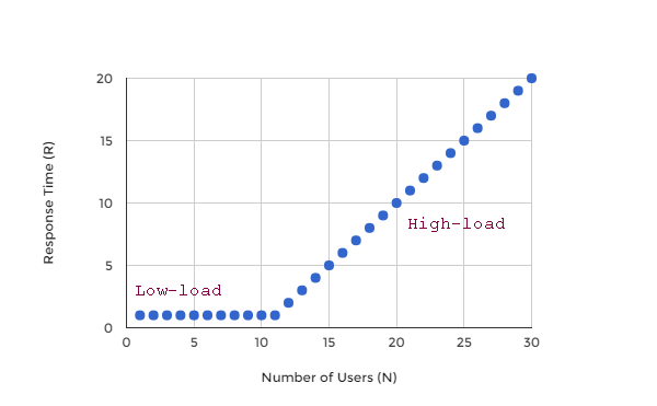
Here are figures showing these relationships. In particular, stop and look carefully at the response time one. The full understanding of this figure is capital and, according to my experience, it is not widely known.

In the Real World
In the real world the R(N) relationship is not so clean, so straight, but the lines shaping it are present there as tendencies.
Light load phase: there are few users, most of the time the server is idle, and when a user arrives is very likely to find it idle, so he does not have to wait
When N⟶0, then R⟶S
|
Transition: if the user population increases, the probability of the server busy, and of queueing, also increases
When N growths, then W growths (R growths)
|
Heavy load phase: In a heavily used service center most of the time the server is busy. is very unlikely to find it idle, so users will have to wait, and users will have to wait more as more users are in the system.
When N⟶∞, then R⟶∞ with ∆R/∆N⟶1/S
|
Coming Next
Applying all this to a SAPS benchmark.
Blog URL: http://www.ibm.com/blogs/performance
Mirror blog: http://demystperf.blogspot.com