Phases of the Response Time

Let us consider a fixed (closed) population of users interacting with a service center, as shown in the following picture below:

1. At t=0, an user arrives to the service center,
2. From t=0 to t=W the user waits in the queue if all the servers (or workers) are busy at t=0,  W is the wait time.
3. At t=W one server gets free and takes the user for servicing him.
4. From t=W to t=W+S and the server gives him the requested service. S is the service time.
5. At t=W+S the user exits the service center after having being serviced.
6. From t=W+S to t=W+S+Z the user remains out of the service center. Z is called the think time.
7. At t=W+S+Z the user goes to step #1. that is, he arrives again at the service center, and the cycle repeats.

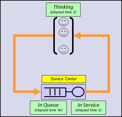
The think time (Z) is a measure of the user activity. It typically is much greater than the Service Time (Z>>S). For example, in SAPS benchmarks Z=10 s and S is about tens of milliseconds. In the context of SAP system sizing high activity users are assigned a Z=10s,  medium activity users Z=30s, and  low activity users Z=300s.

A quantitative approach

The fundamental question we would like to answer is: what is the response time (R) when the user population is N? That is, what is the relationship between the response time and the number of users R=R(N).

To focus on principles, and to keep things simple, let's derive R(N) with the simplifying assumptions:

• S is constant,
• Z is constant.
• m=1 (It is easily generalizable to an arbitrary number of workers).

Light Load Phase

Let us suppose there is only one user, that is, total population number is equal to one (N=1). The lone user arrives to the service center, never queues, receives service, departs, is away, and comes back to the service center.  This loop is periodically repeated, being the period Z+S (the time it takes the user to cycle once round the "loop"). The lone user never meets anyone, never queues. In this case Q=0, W=0 and R=S. The system throughput is 1/(Z+S).

Let's add another user to the system (N=2). It could happens that both users arrive at the same time to the service center, and in such a case one is immediately served and the other waits until the first is finished being served (remember that m=1). But at the next loop neither of them will have to wait, because the second user has been  delayed by S the first time through. So after the initial transitory interval there are nobody queued, never, Q=0, W=0 and R=S. The system throughput is 2/(Z+S).

The same will happen with an increasing population number, N=3, 4... but, until how many users?

The Phase Transition

How many users can the system support without queueing (except in the initial transitory phase)? We call this specific value the saturation population, or saturation point, and it will be identified by N*. It's easy to calculate that

N*=1+Z/S

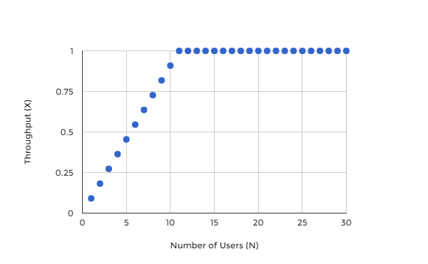
At the saturation point the throughput is N*/(Z+S)=1/S.

Heavy Load Phase

Above the saturation population (N>N*) the light-load equilibrium radically changes: we cannot add additional users and keep the number in the queue (Q) equal to zero.

Add the N*+1 user. Let's suppose, without losing generality, that this additional user (CN*+1) arrives at the service center in some point within the time interval where user 1 (C1) is receiving service. As the server is busy with C1, then CN*+1 has to wait. When C1 exits, CN*+1 is taken by the server for service. But at this very moment user C2 comes back from the Think state, and surprise! he finds the server busy and has to wait! (until now when coming back he didn't have to wait). C2 has to wait exactly S units of time, the service time for the CN*+1 user.

When the server releases user CN*+1 , it takes C2 from queue, and C3 comes back seeking for service. C3 find "his" time slot occupied by C2 and has to wait S units of time in the queue (W=S). And this pattern repeats for every other user. All users have to wait S units of time in queue (W=S)!  For a population of N*+1 users there's always a user queued (Q=1), the wait time W is equal to S (W=S), and the response time equals to 2S (R=W+S=2S).  The throughput remains the same, 1/S, that is, adding one user does not increase the throughput.

The same analysis may be performed with another additional user, the CN*+2, just to obtain that in such a case there will always be two queued users (Q=2), the wait time for all users will be W=2S, and response time for all users will be R=2S+S=3S. The throughput remains 1/S.

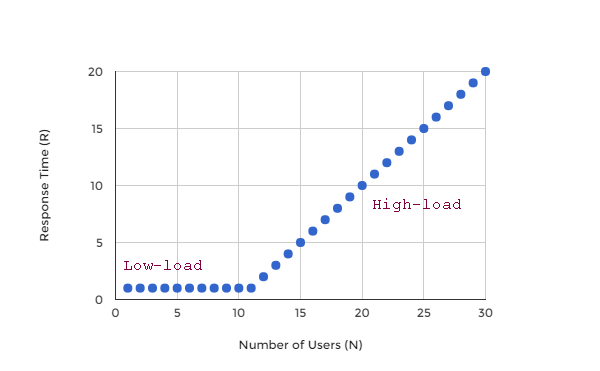
Applying the same reasoning It’s trivial to conclude that when the user population is N users (N>N*), the queue size will be Q(N)=N-N*, the wait time in queue is W(N)=S·(N-N*), and the response time R(N)=S·(1+(N-N*)).

The situation has radically changed when going above the saturation point! From an idyllic response time when below the saturation point, to an increasing response time with each additional user above the saturation point.

The Complete Relationship R(N)

The following table Table summarizing our findings so far:

	Light Load (N<=N*)	Heavy Load (N>N*)
N*	N*=1/(Z+S)
Q(N)	0	N-N*
W(N)	0	S·Q
R(N)	S	S+W(N)
X(N)	N/(Z+S)	1/S

Here are figures showing these relationships. In particular, stop and look carefully at the response time one. The full understanding of this figure is capital and, according to my experience, it is not widely known.

In the Real World

In the real world the R(N) relationship is not so clean, so straight, but the lines shaping it are present there as tendencies.

Light load phase: there are few users, most of the time the server is idle, and when a user arrives is very likely to find it idle, so he does not have to wait

When N⟶0,  then  R⟶S

Transition: if the user population increases, the probability of the server busy, and of queueing, also increases

When N growths,  then  W growths  (R growths)

Heavy load phase: In a heavily used service center most of the time the server is busy. is very unlikely to find it idle, so users will have to wait, and users will have to wait more as more users are in the system.

When N⟶∞,  then  R⟶∞  with ∆R/∆N⟶1/S

Coming Next

Applying all this to a SAPS benchmark.

---

Blog URL:   http://www.ibm.com/blogs/performance
Mirror blog:  http://demystperf.blogspot.com

More or Faster?

The More or Faster dilemma

What would you choose? MORE  but slow workers or to have fewer but FASTER workers?

Let's explore a little bit to find an answer.

Hairdresser’s

You have the opportunity to choose between two hairdresser's that have advertised, and it's true indeed, they are capable of 4 haircuts per hour:

• The Faster with only 1 worker (m=1) and 15 minutes service time (S=15min),
• The More with 4 hairdressers (m=4) and 1 hour service time (S=1h).

If just before entering you see a queue of 5 (Q=5) in both shops, which one should you choose?

Response:

• The More: the response time, the total time you'll spend there, is between 2 h and 3 h,

• The Faster: the response time, the total time you'll spend there, is between 1 h 30 min and 1 h 45 min.

It's better to choose "The Faster".

Company Department

The scheduling manager has to decide which department to send incoming jobs to. She has to make a choice between two departments delivering the same maximum performance (2 jobs per day).

• The Faster department with 4 experienced and very efficient professionals (m=4) spending  2 days per job (S=2d).
• The More department with 8 less experienced people (m=8) who spend 4 days per job (S=4d).

If the queue is 10 jobs long (Q=10)  in both departments, what should she choose?

Response:

• The More: the next incoming job would take between 24 and 28 days to be processed.
• The Faster: the next incoming job would take between 12 and 14 days to be processed.

It's better to choose "The Faster".

Below is the plot of the response time I see against the number in the queue (Q) for "The Faster" (red)  and "The More" (yellow)  alternatives in the hairdresser's case. It cleanly illustrates that "The Faster" is better, because of the delivered response time is smaller.

Learning point: given the same bandwidth (maximum throughput) always choose the service center with the fastest workers.

---

New blog URL:   http://www.ibm.com/blogs/performance

Mirror blog:  http://demystperf.blogspot.com

How much do I have to wait?

Wait time is lost time

I suppose everyone agrees with the sentence: wait time is lost time. Nobody likes or wants to wait. From the customer (requester) point of view wait time is, in general, badly tolerated.

But the service provider point of view is different. In general it would not provide ample capacity to eliminate any waits, given that the capacity has a cost and probably will remain idle out of peak times. An agreement/equilibrium must be reached.

How much do you have to wait?

Suppose you are a customer, arrive to a service center that has one worker, and find Q customers waiting in the queue ahead of you, and one customer being serviced. How much do you have to wait?

The response is simple: the remaining service time for the customer being serviced, plus the service time of the 1st customer in the queue, plus the service time for the 2nd customer in the queue,..., and so on until the last customer  queued (the number Q). This results in the following expression for the waiting time (W) ():

S1 + S2 + ... + SQ  <=  W  <=  S0 + S1 + S2 + ... + SQ

If we make the simplifying assumption that the service time (S) is constant, that is, every customer spends the same amount of time receiving service, we have this simpler expression

Q · S  <=  W  <= (Q+1) · S

and being the response time equal to the sum of the waiting time and the service time (R = W + S) we have

(Q+1) · S  <=  R  <= (Q+2) · S

In the case of a service center that has m workers, and S constant, the bounds to the waiting and the response time are

S*INT(Q /m)  <=   W   <=  S+S*INT(Q /m)

and

S + S*INT(Q /m)  <=   R   <=  2S + S*INT(Q /m)

where INT() is the integer part function.

So the waiting time depends on:

• The Service Time  (S):  If the service time, mine or of the customers ahead in the line, increases (decreases) the response time will increase (decrease) as well.
• The Number of Workers  (m): If the number of workers increases (decreases) the wait time will decrease (increase) as the line will advance faster (slower).
• The number of queued customers (Q), that is, the number of waiting (queued) customers ahead of you. The bigger Q is the bigger the wait time is.

Practical cases

Hairdresser’s:

My hairdresser’s has the following performance values: a service time of 1 hour (S=1 h), and four hairdressers at work (m=4). When I arrive there, willing to get an haircut, there are 4 customers in the waiting room (Q=4).

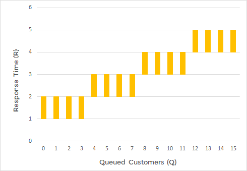
I can easily derive that I'll have to wait between 1 and 2 hours,  as  1*int(4/4)=1  and 1+1*int(4/4)=2. That is, the response time I will experience will be between 2 h and 3 h.

Here is the plot of the response time (R)  interval against the number in the queue (Q):

Company Department:

In my company department jobs take one working day to be completed (S=1 day), and there are three equally qualified professionals working there  (m=3). So when a new job arrives and "finds" a queue of 6 (Q=6), it may be concluded that the job requester must have to wait between 3 and 4 days to get his request serviced, as 1 + INT(6/3) <= R <= 2 + INT(6/3).

---

New blog URL:   http://www.ibm.com/blogs/performance

Mirror blog:  http://demystperf.blogspot.com

Introducing the Response Time

Introducing the Response Time

The response time is the loser in the set of all performance metrics. It's systematically ignored in almost every sizing, it’s neither measured nor accounted in most cases, and it's only marginally referenced in certain benchmark definitions. Clearly, the throughput is the winner: SAPS, IOPS, transactions per second are throughput metrics, not response time ones.

But from the end user point of view the response time is the king. Any service center performs very well or very poorly according to the response time perceived by its users. When the response time is bad It doesn't matter to the customers if the system administrator proclaims they are working with a many-oooops-per-second system. Just the system is slow and, consequently, bad. Period.

The Service Center

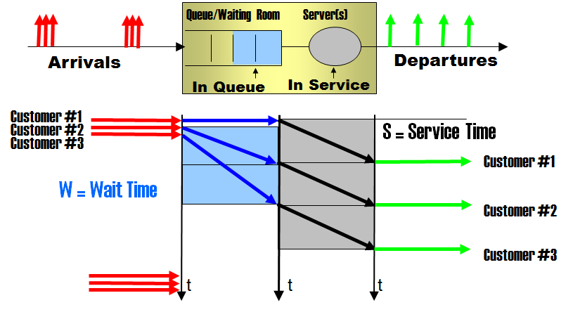
Look at the following picture, an idealization of any service center. A service center is a place, logical or physical,  where customers or users enter, are given a certain service by a worker (or a server), and exit. There's a line (queue) where arriving customers can queue and wait if all the workers are busy.

Figure: Service center with server(s), queue, and arriving  and departing customers.

You interact with service centers everywhere, as it is very general concept. For example:

Service Center	Service Given	Customer	Worker
Hairdresser’s	A haircut	People needing a haircut	Hairdresser
Our Company department	A step in an opportunity forward path	Company customers	Yourself
OLTP IT Server	CPU time	Users entering transactions at their terminals	CPU cores
Supermarket checkout	The checkout payment	Supermarket customers	Cashier
Bus Transport	A transport from place A to place B	Passengers	The driver and the bus
Public office desk	A request to the public administration.	Citizens	Public servant
Machine Repair Center	Fixing the malfunctioning machine	Machines	Repairman

A service center is fully characterized by the following magnitudes:

• The service time (S): the elapsed time a service takes,
• The number of servers (m):  the number of customers that can receive service simultaneously.

The Response Time

The Response Time (R) is the time elapsed from the arrival of a customer to the service center to its departure after receiving service.

The response time has two contributions: the service time (S)  and the wait time (W), resulting in this fundamental relationship:

R = W + S

To illustrate this look at the following scenario where we have depicted the flow of several customers through a very simple service center (m=1, S=cte)

• Customer #1  arrives a t=0, finds the worker/server idle, spends no time at all at waiting, is given a certain service taking S units of time, and exits the center of service at t=S. The wait time is 0. The response time is S.
• Customer #2  arrives a t=S, spends no time at all waiting, is given a certain service taking S units of time, and exits the center of service at t=2S. The wait time is 0. The response time is S.
• Customer #3  arrives a t=2S, spends no time at all waiting, is given a certain service taking S units of time, and exits the center of service at t=3S. The wait time is 0. The response time is S.

In this scenario none of its customers must wait for service, and so the response time is equal to the service time. The wait time contribution is zero.

Now look at the following scenario differing from the previous one in the way customers arrive.

• Customer #1  arrives a t=0, spends no time at all at the queue, is given a certain service taking S units of time, and exits the center of service at t=S. The wait time is 0. The response time is S.
• Customer #2  arrives a t=0, has to wait in queue S units of time, is given a service taking S units of time, and exits at t=2S. The wait time is S. The response time is 2S.
• Customer #3  arrives a t=0, has to wait in queue 2S units of time, is given a service taking S units of time, and exits at t=3S. The wait time is 2S. The response time is 3S.

Some of the customers must wait for service and, consequently the response time has the two contributions: the service time (grey) and the wait time (blue),

Waiting for the SAPS

Looking at a SAPS benchmark report, may you tell which contribution to the response time is bigger: the wait or the service time?

Remember this first: SAPS is a performance metric measuring throughput: 1 SAPS is 1 customer service per minute, or 1 dialog step per minute (dialog step is an SAP term). The benchmark is essentially performed by progressively increasing the customer population, and monitoring the response time.  When the response time reaches 1 second (R=1 s), the measured throughput, as expressed in dialog steps per minute, is the SAPS value.

A SAP server in essence is a service center for SAP dialog steps. And according to the certification report these are its measured numbers:

• There are 128 workers, corresponding to 128 HW threads executing dialog steps, so m=128.
• The average response time is measured to be 0.98 s. R=0.98 s.
• 5113000 dialog steps are executed (serviced) in an hour.

And from the above the following values can be easily derived:

• The service time is S=0.090 s , as every worker processes (5113000/128) ds per hour, and then  ( 1 h / (5113000/128) ds ) · ( 3600 s/h) = 0.0901 s.
• The wait time is W= 0.89 s  (W = R - S).

The dialog step response time is decomposed into 0.89 s of wait time and 0.09 s of service time:

Wow!  W >> S, in fact W ~ 10·S. So it’s sure there is a queue of dialog steps waiting  to be processed. If you scale this to, for example, a supermarket checkout counter that spends  5 minutes per customer, W=10·S means a 50 minutes waiting in the line!

Coming Soon

This is the first blog entry of the Demystifying the Response Time series, an exploration into the response time jungle. There are very interesting facts and analysis ahead. Stay tuned.

---

New blog URL:   http://www.ibm.com/blogs/performance

Mirror blog:  http://demystperf.blogspot.com